Spectral Unmixing
Spectral unmixing🔗
The Spectral unmixing tool is used to separate an image into its component spectra. The user selects a set of spectra, termed "endmembers", from the project, and the chosen algorithm will generate abundance maps for each spectrum. These maps represent the contribution of each endmember to the input pixel.
Warning
Unmixing requires access to Compute.
Background🔗
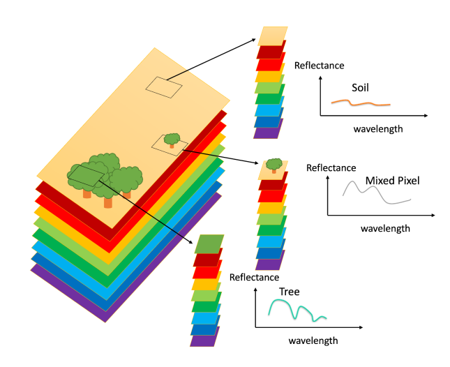
Depending on the resolution of the data, most of the pixels in a remote sensing image will be "mixed," meaning they contain information from several different materials. The spectrum of the resulting pixel can be represented as a weighted sum of the spectra for all materials present in the pixel, with the weights representing the proportion of each material. Unmixing, then, is the process of recovering the weights given an image and a set of endmember spectra. The image above, from here, shows a simple example of pure versus mixed pixels.
Tip
Proper selection of endmember spectra is the most important step of the unmixing process.
Selecting data🔗
The unmixing dialog allows you to choose the raster layer and bands to use as input data, and spectra to use as endmembers.
Note
Spectra will be automatically resampled to the data wavelengths if necessary.
Output layer🔗
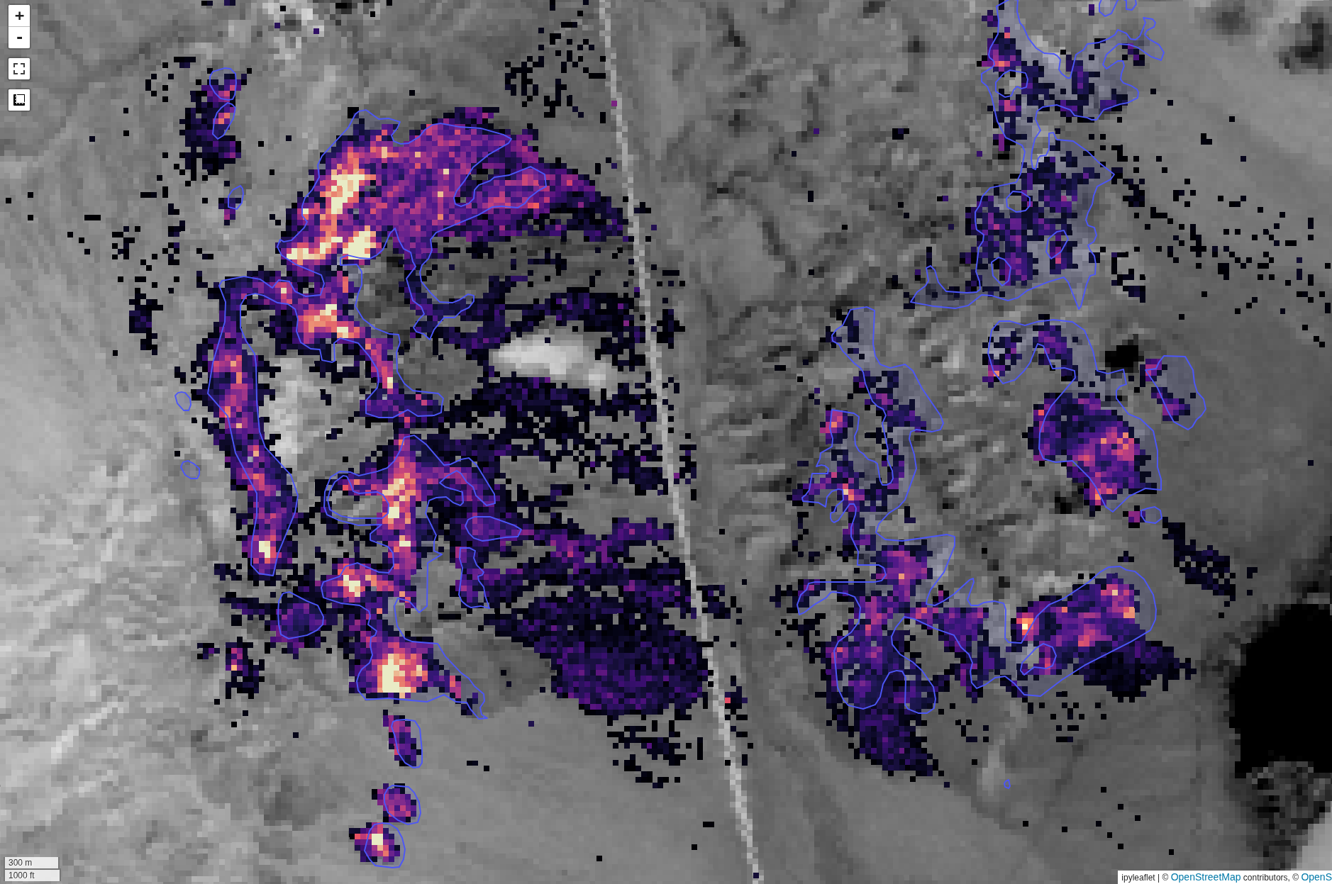
The output layer that is generated will have one band per endmember spectrum, representing the relative abundance for each endmember. The above image shows an example output from the Cuprite region for Alunite, compared with an interpretation from ground truth data (ground truth from here)
In addition, an error band is generated, representing the RMS error between the input image and the image as reconstructed by the abundance maps.
Unmixing parameters🔗
Several parameters are available to control the unmixing process.
Method🔗
Least squares🔗
 Solve the mixture problem via a least-squares optimization. Background for this method
is available here.
Solve the mixture problem via a least-squares optimization. Background for this method
is available here.
Distance geometry-based🔗
 Utilizes a geometry-based restating of the unmixing problem. Background is available
here
Utilizes a geometry-based restating of the unmixing problem. Background is available
here
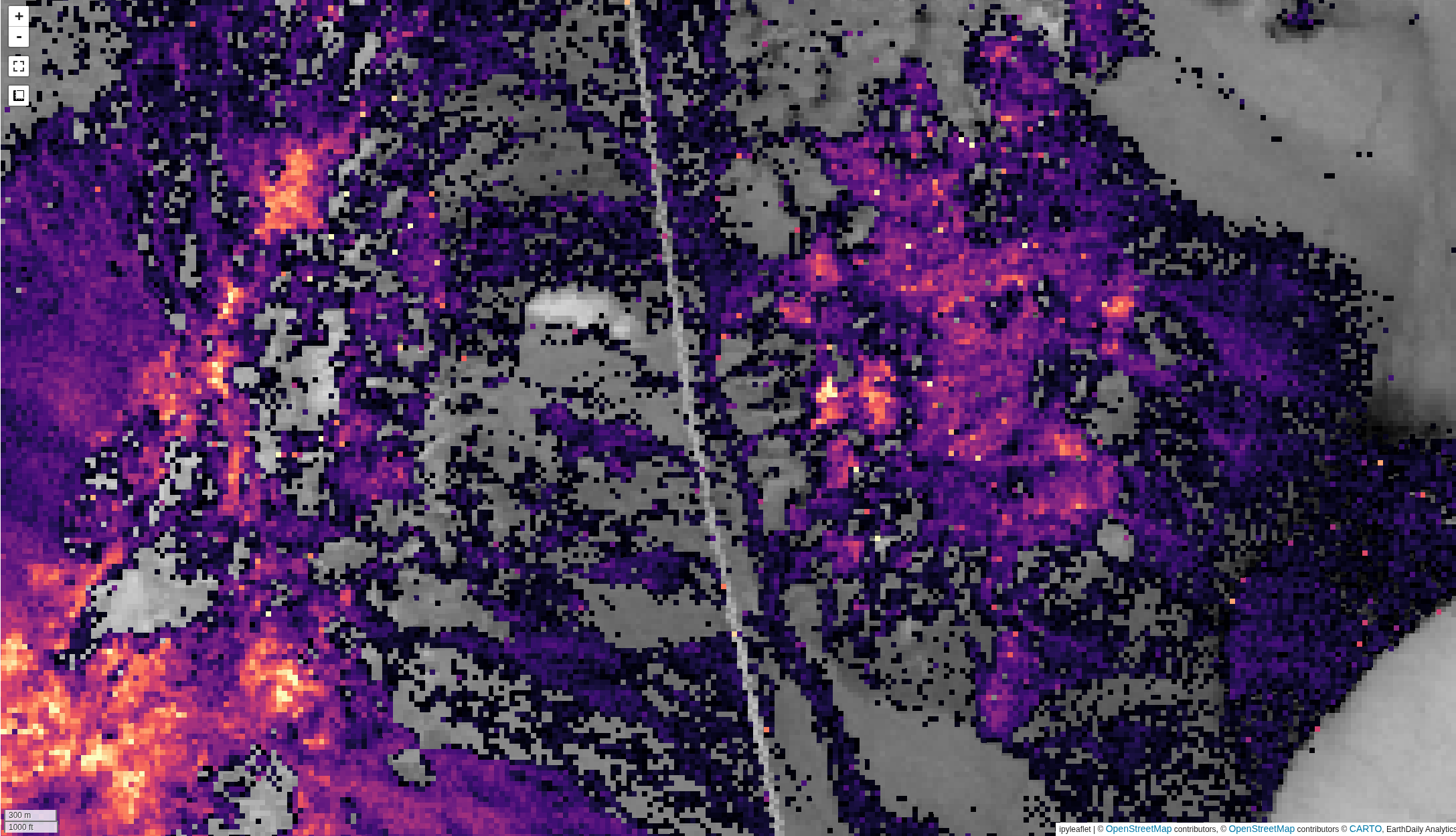
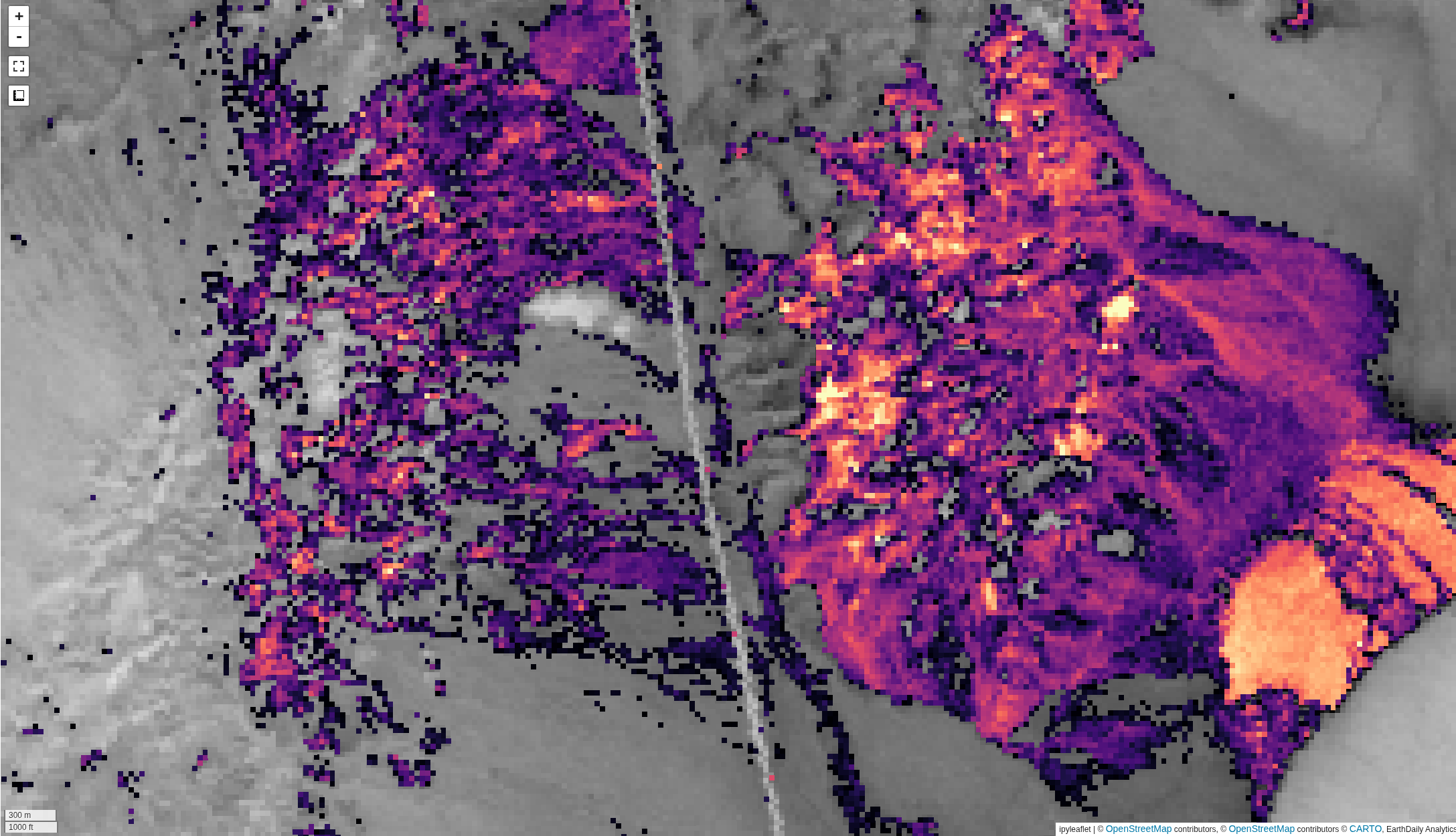
Hull normalization🔗
Applies a hull normalization process to the data and spectra before unmixing. This is useful for matching the shapes of the spectra, without concern for amplitudes.
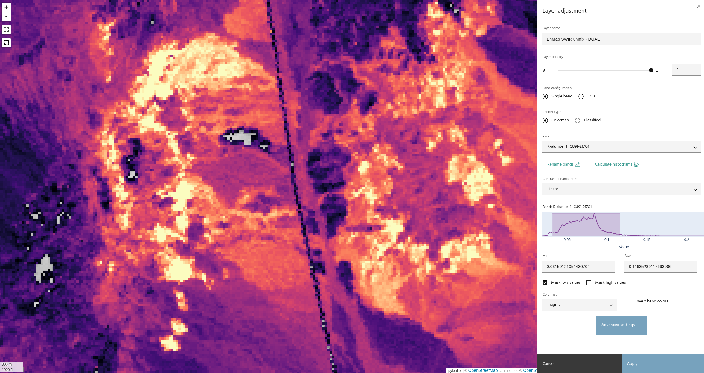
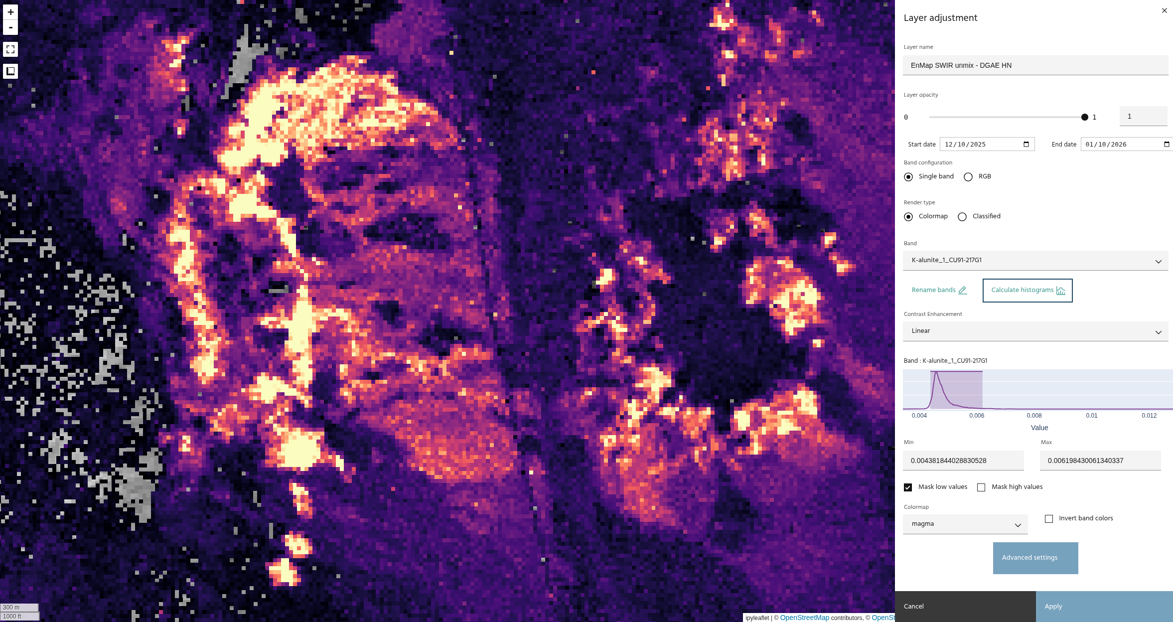
The images above compare unmixing without (top) and with (bottom) hull normalization. Note that the results have similar trends, with a much tighter histogram on the normalized data.
Constraints🔗
Two constraints for the solution are available:
- Non-negativity: Ensures that all abundance maps are strictly positive
- Sum-to-one: Ensures that the abundance maps all sum to one. This allows a physical interpretation of the abundance maps as true mixture percentages.
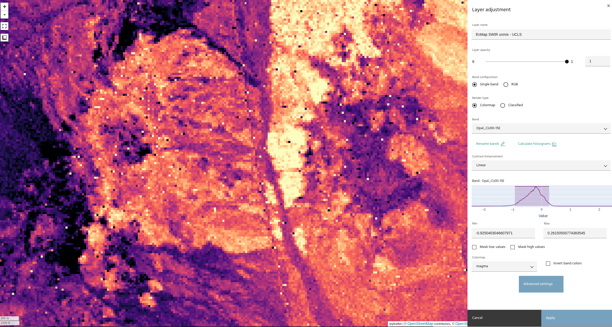
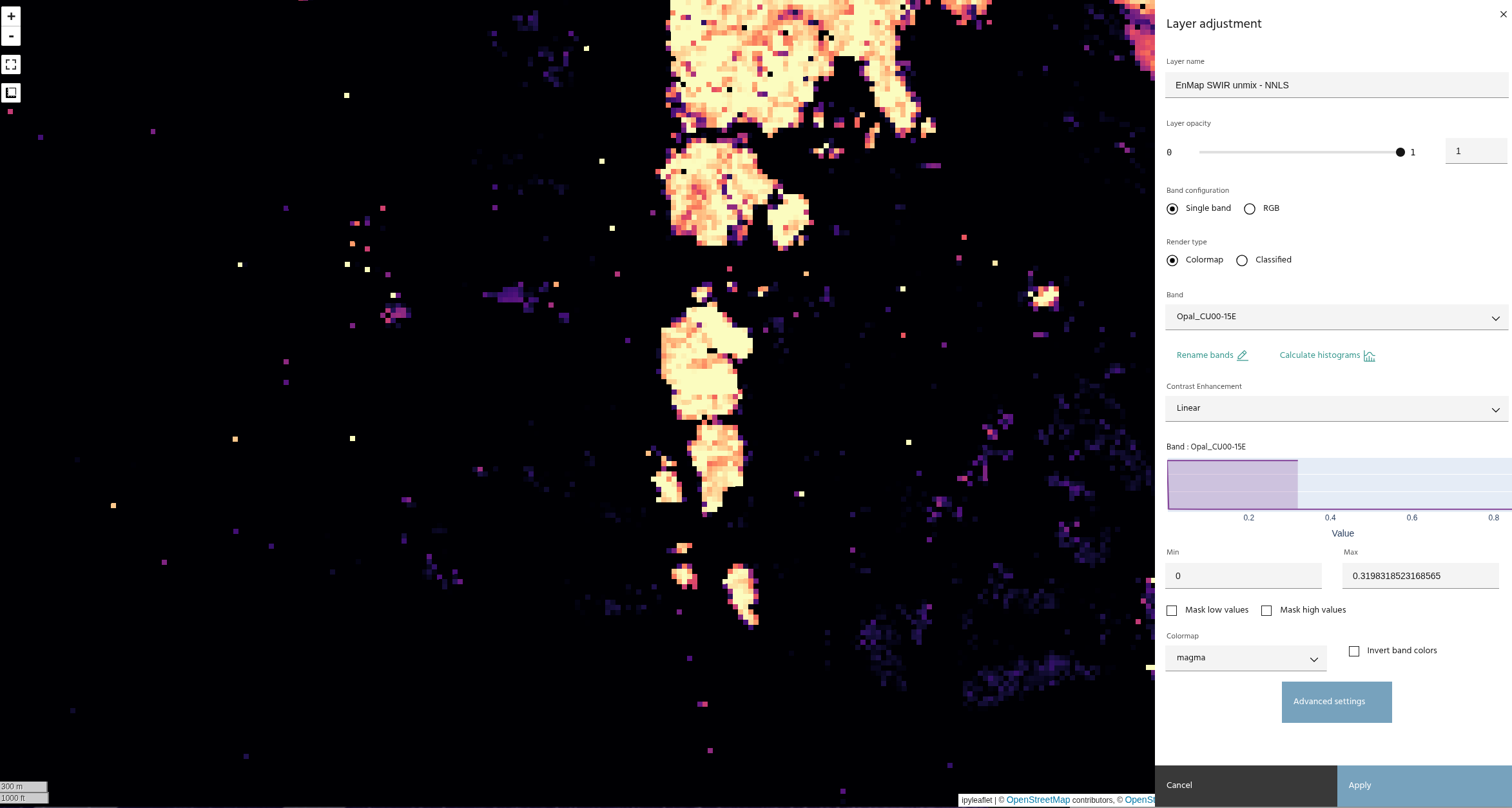
These images show the difference between an unconstrained least squares and the non-negativity constraint.
Note
Constraints are not selectable with Distance geometry-based unmixing, as the constraints are built into the method.